Build an ML model to predict YouTube video views

Hands-on end-to-end ML project for the busy learner – Part III

Tamás Ujhelyi

Nov 16, 2024

Got a nice dataset?

Good for you.

Now make it good for the business, too.

Scratch that itch, train your machine learning (ML) model, and – more importantly – prove its worth.

In Part III of this series, here’s what you’ll get to do:

calculate a baseline performance your ML model needs to beat,
build an XGBoost and a LightGBM model to predict YouTube video views,
evaluate your ML models against the baseline using error metrics,
and modify your dataset to improve your ML models’ performance.

If you read this article, I’ll assume you’ve completed Part I and Part II; if not, please go through those articles first since this tutorial heavily builds on them.1

I’m also assuming you’re familiar with data science basics like splitting a dataset into train and test sets, and understanding features vs. targets.

If you’ve nailed these prerequisites, you’re more than qualified to continue reading.

Oh, and here’s the link to the repo.

1. A high-level overview of what the script does

By the end of this article, you’ll have this up and running:

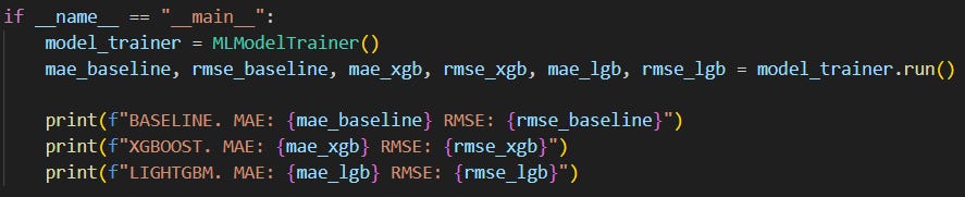
It may not seem much (it’ll be a LOT, though), but it’s honest work.

The script:

creates model_trainer containing everything to build the machine learning models,
evaluates the models’ performance,
and prints the evaluation results to compare them against a baseline, no-ML solution.

(I could show you a screenshot of what’s coming, but hey, no spoilers!)

But what’s inside model_trainer.run()? 🤔

It’s quite a bit.

Check it out real quick, but don’t stress about understanding it just yet:

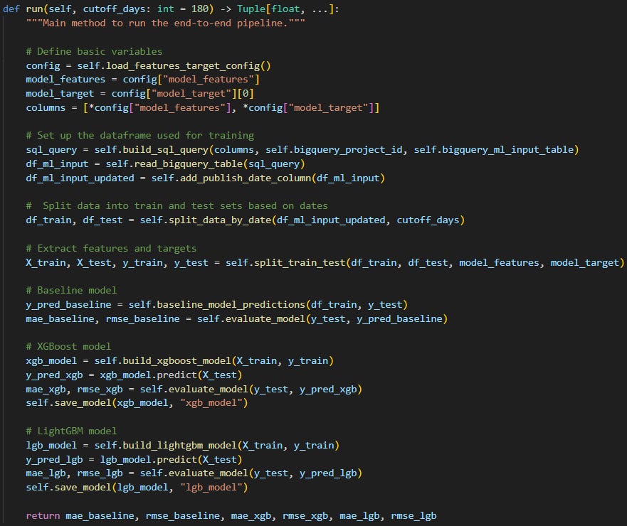
So run():

defines the features and the target variable ML models will use for training (# Define basic variables),
loads the YouTube dataset (created in Part II) from BigQuery into a dataframe with some minor additions (# Set up the dataframe used for training),
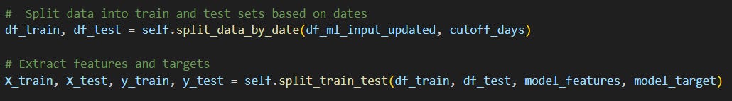
divides the loaded dataset into a train and a test dataframe (# Split data into train and test sets based on dates) and separates the features from the target variable (# Extract features and targets),
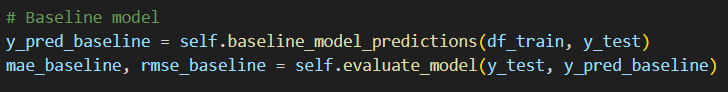
calculates a baseline performance without any ML so we can check if we need ML at all (# Baseline model),
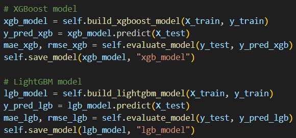
trains an XGBoost (# XGBoost model) and a LightGBM ML model (# LightGBM model),
calculates the baseline’s and the two ML models’ performance measured by two error metrics: mean absolute error (MAE) and root mean squared error (RMSE).

All this hustle just to pick the best solution (baseline or any of the ML models).

Now, let’s build this stuff!

2. A detailed explanation of how the script works

As you’ve seen, MLModelTrainer() is responsible for everything.

It has fifteen methods dealing with different parts of model building and evaluation.

We’ll check them out one-by-one.

(I’ve removed the docstrings from the method explanations to spare you some unnecessary scrolling).

2.1 The “init()” method

def __init__(self) -> None:

        # Load environment variables
        load_dotenv()

        self.bigquery_project_id = os.getenv("BIGQUERY_PROJECT_ID")
        self.bigquery_ml_input_table = os.getenv("BIGQUERY_ML_INPUT_TABLE")
        self.credentials = service_account.Credentials.from_service_account_file(
            "service-account-key.json"
        )

        # Check for presence of required environment variables
        if not all([self.bigquery_project_id, self.bigquery_ml_input_table, self.credentials]):
            raise ValueError("Missing required environment variables.")

The __init__() method:

loads your BigQuery credentials and the necessary environment variables,
checks whether all required environment variables are present; if not, an error is raised.

2.2 The “load_features_target_config()” method

def load_features_target_config(self, config_path: str = "features_target_config.yaml") -> Dict[str, List[str]]:
  
        with open(config_path, "r") as file:
            config = yaml.safe_load(file)
        
        return config

Honestly, this is one of my favorite parts of the script.

The load_features_target_config() method:

loads a yaml file listing the feature names and the target variable so other parts of the script can easily refer to them.

This solution has two major advantages:

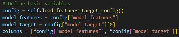
we don’t have to list the feature names in our script to use them (e.g. in a SQL query); it’s simply enough to assign config[“model_features”] to a variable and refer to that like here:
it makes it easier to manage the list of the features and the target variable, because everything can be set up/modified in the yaml file, which means no more rewriting in the script.

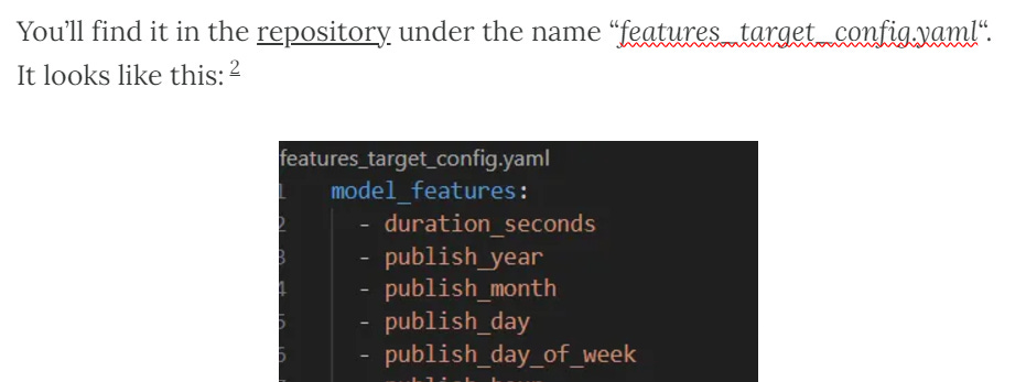
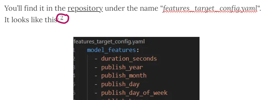
But where is this yaml file?

You’ll find it in the repository under the name “features_target_config.yaml“. It looks like this:2

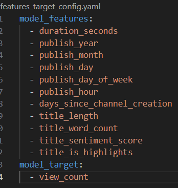
Later on we’ll make good use of this file so don’t forget about its existence!

2.3 The “build_sql_query()” method

def build_sql_query(self, columns: List[str], bigquery_project_id: str, bigquery_table: str) -> str:

        columns_str = ", ".join(columns)
        
        return f"""
        select
            {columns_str}
        from
            `{bigquery_project_id}.{bigquery_table}`
        """

The build_sql_query() method:

builds a SQL query that’ll be used to query the ml-input table from BigQuery (remember: this table holds the features and the target variable that we created in the previous article).

A sneak peek: columns contains the column names (=features (e.g. duration_seconds) and target variable (view_count)) that we select in our SQL query.

columns is created with the help of the yaml file we’ve just discussed:

Neat, isn’t it? 😉

2.4 The “read_bigquery_table()” method

def read_bigquery_table(self, sql_query: str) -> pd.DataFrame:

        df = pandas_gbq.read_gbq(
            sql_query,
            project_id=self.bigquery_project_id,
            credentials=self.credentials
        )

        return df

The read_bigquery_table() method:

uses the SQL query generated by build_sql_query() and loads the query’s result from BigQuery into a pandas dataframe.

2.5 The “add_publish_date_column()” method

def add_publish_date_column(self, df: pd.DataFrame) -> pd.DataFrame:
        
        df_copy = df.copy()
        
        df_copy["publish_date"] = pd.to_datetime(
            dict(
                year=df_copy["publish_year"], 
                month=df_copy["publish_month"], 
                day=df_copy["publish_day"]
            )
        )

        return df_copy

The add_publish_date_column() method:

uses the publish_year, publish_month and publish_day columns from the previously loaded dataframe by read_bigquery_table(),
to add a new column (publish_date) by combining the columns (e.g. 2024, 10, 01 will be transformed into 2024-10-01),
and creates a new dataframe containing the original columns and a new one (publish_date).

The script later will use publish_date to determine at which date to split the dataset into train and test datasets (see the next methods).

We need this column to do a time-based split instead of just randomly splitting the data:

the earlier time period will contain the training data (e.g. between 2023-01-01 - 2024-03-31),
the later time period will contain the test data (e.g. between 2024-04-01 - 2024-10-31).

2.6 The “find_cutoff_date()” method

def find_cutoff_date(self, df: pd.DataFrame, cutoff_days: int = 180) -> pd.Timestamp:
        
        # Calculate the cutoff date (n days before the latest date in the dataset)
        latest_date = df["publish_date"].max()
        cutoff_date = latest_date - timedelta(days=cutoff_days)
        
        return cutoff_date

The find_cutoff_date() method:

finds the date based on which an other method (split_data_by_date()) will divide the dataset into a train and a test set,
and it does so by receiving the whole dataset as input,
and finding the cutoff date based on the number of days you provide (default value is 180 which is around 6 months),
so for instance if you find it reasonable based on your dataset that the most recent 120 days should be used for testing, you’d assign 120 to cutoff_days.

2.7 The “split_data_by_date()” method

def split_data_by_date(
        self,
        df: pd.DataFrame,
        cutoff_days: int
    ) -> Tuple[pd.DataFrame, pd.DataFrame]:
        
        df_copy = df.copy()
        cutoff_date = self.find_cutoff_date(df_copy, cutoff_days)
        
        # Create train and test DataFrames based on the cutoff date
        df_train = df_copy.query("publish_date <= @cutoff_date").reset_index(drop=True)
        df_test = df_copy.query("publish_date > @cutoff_date").reset_index(drop=True)
        
        return df_train, df_test

The split_data_by_date() method:

uses the cutoff date identified by find_cutoff_date(),
and divides the dataset into a train and a test dataset; anything after the cutoff date (e.g. 2024-10-01) goes into the test dataset (e.g. beginning from 2024-10-02) and everything else goes into the train dataset (e.g. 2024-10-01, 2024-09-30, etc.).

2.8 The “split_train_test()” method

def split_train_test(
            self,
            df_train: pd.DataFrame,
            df_test: pd.DataFrame,
            model_features: List[str],
            model_target: str
    ) -> Tuple[pd.DataFrame, pd.Series, pd.DataFrame, pd.Series]:
        
        X_train = df_train[model_features]
        X_test = df_test[model_features]
        y_train = df_train[model_target]
        y_test = df_test[model_target]

        return X_train, X_test, y_train, y_test

The split_train_test()3 method:

takes the train and test datasets created by split_data_by_date(),
reads the features and target variable defined in features_target_config.yaml,
and divides the data into the usual four sets used for ML model building and testing: X_train, X_test, y_train and y_test.

2.9 The “evaluate_model()” method

def evaluate_model(self, y_true: pd.Series, y_pred: List[float]) -> Tuple[float, float]:

        mae = mean_absolute_error(y_true, y_pred)
        rmse = root_mean_squared_error(y_true, y_pred)
        
        return mae, rmse

The evaluate_model() method:

calculates the performance of the ML models,
by using two different error metrics: mean absolute error and root mean squared error.

If you’re not familiar with these error metrics, I highly recommend to watch this explanation video.

2.10 The “calculate_baseline()” method

def calculate_baseline(self, df_train: pd.DataFrame, days: int) -> int:
        
        # Calculate the cutoff date (n days before the latest date in the dataset)
        latest_date = df_train["publish_date"].max()
        cutoff_date = latest_date - timedelta(days=days)
        
        # Filter data to only include the past n days
        recent_data = df_train[df_train["publish_date"] > cutoff_date]
        
        if not recent_data.empty:
            return round(recent_data["view_count"].mean())
        else:
            raise ValueError("No data available for the past n days.")

The calculate_baseline() method:

takes the train dataset (df_train) and number of days (days) as input,
to calculate the average of the target variable (view_count) overt the past, most recent n days (e.g. 30),
by first finding the latest date (e.g. latest_date = 2024-10-31) in the train dataset,
and identifying a cutoff_date (e.g. 2024-10-01) to filter the train dataset to contain only the past n days (recent_data; e.g. 2024-10-02 - 2024-10-31, which is 30 days),
to finally calculate the mean value for view_count for the past n days.

As you’ll see, the next method (baseline_model_predictions()) will use this calculated baseline as the predicted view_count for each video.

For instance, if the baseline prediction is 500 000 views, then the baseline model predicts that no matter what, a newly uploaded video is likely to receive 500 000 views.

Using the average of historical data (=df_train) as a prediction is a common way when working with time-based data.

The only modification I’ve made here is that the script calculates the average based on the past n days instead of the whole train dataset, because I find it more realistic in this use case.

But again, you can change this to any number by using days in the next method (baseline_model_predictions()).

2.11 The “baseline_model_predictions()” method

def baseline_model_predictions(self, df_train: pd.DataFrame, y_test: pd.Series, days: int = 30) -> List[float, ...]:

        baseline_value = self.calculate_baseline(df_train, days)
        predictions = [baseline_value] * len(y_test)

        return predictions

The baseline_model_predictions() method:

takes the baseline prediction value calculated by calculate_baseline(),
and assigns this prediction to each row (=video) in the train dataset (e.g. if the train dataset contains 800 rows, we’ll have 800 baseline predictions: the exact same prediction for each row),
and returns this in a list (predictions).

The script basically imitates an ML model that generates predictions for each row in the y_train dataset, but it’s not actually an ML model – it just repeats the same prediction for every row in y_train.

Once we have predictions, the performance of the baseline model can be measured, and the ML models we’ll create with the next methods will have to beat this performance to prove worthy of using (otherwise we’ll go with the baseline solution).

2.12 The “build_xgboost_model()” method

def build_xgboost_model(self, X_train: pd.DataFrame, y_train: pd.Series) -> xgb.XGBRegressor:

        model = xgb.XGBRegressor()
        model.fit(X_train, y_train)

        # Feature importance visualization
        fig, ax = plt.subplots(figsize=(8, 4))
        xgb.plot_importance(model, importance_type="gain", ax=ax, title="XGBoost feature importance")
        plt.show()

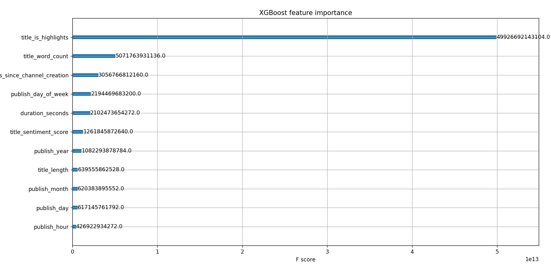
        return model

The “build_xgboost_model()” method:

uses the xgboost library,
to create a basic XGBoost regression model,
and while doing so it also visualizes how important each feature is according to the model in making its prediction:

Why XGBoost (and LightGBM)? I’ve heard from many senior data scientists that these models usually get the best results for tabular data.

That being said, feel free to experiment with other models too. I’m curious what you’ll find!

2.13 The “build_lightgbm_model()” method

def build_lightgbm_model(self, X_train: pd.DataFrame, y_train: pd.Series) -> lgb.LGBMRegressor:

        model = lgb.LGBMRegressor()
        model.fit(X_train, y_train)

        # Feature importance visualization
        lgb.plot_importance(model, importance_type="gain", figsize=(8, 4), title="LightGBM feature importance")
        plt.show()
        
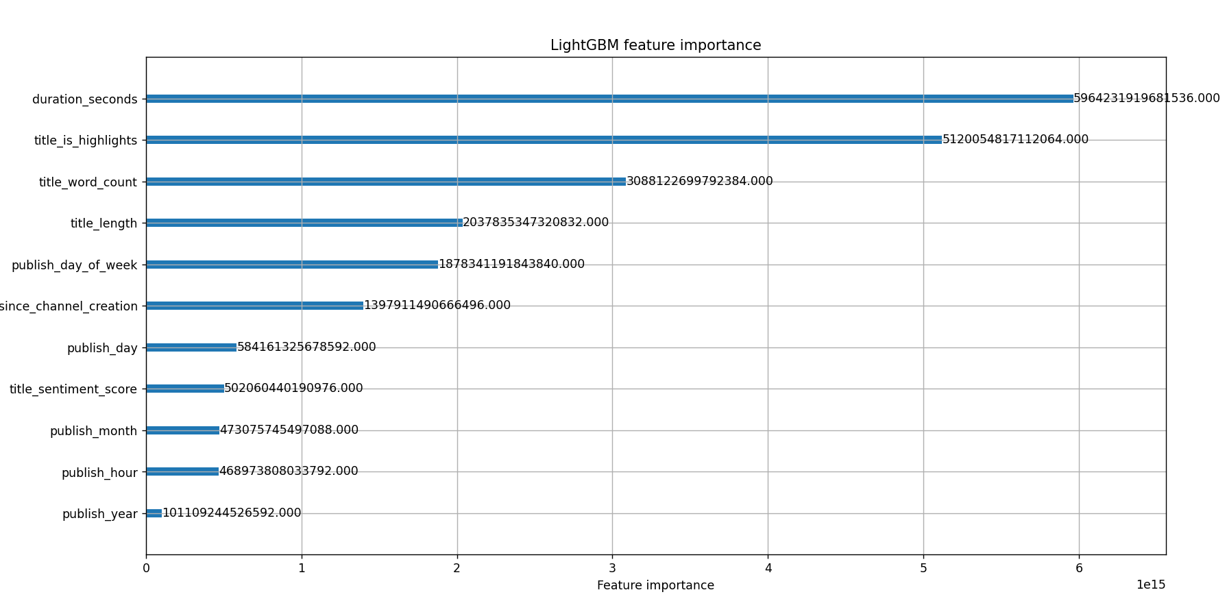
        return model

The build_lightgbm_model() method:

uses the lightgbm library,
to create a basic LightGBM regression model,
and while doing so it also visualizes how important each feature is according to the model in making its prediction:

2.14 The “save_model()” method

def save_model(self, model: Any, filename: str) -> None:

        timestamp_now = datetime.now().strftime("%Y%m%d_%H%M%S")
        filename_with_timestamp = f"{filename}_{timestamp_now}.pkl"
        
        with open(filename_with_timestamp, "wb") as file:
            pickle.dump(model, file)

The save_model() method:

saves the trained ML models into a pickle file for later use,
and names them after the model and the timestamp they were created (e.g. xgb_model_20241012_144716.pkl).

2.15 The “run()” method

def run(self, cutoff_days: int = 180) -> Tuple[float, ...]:
        """Main method to run the end-to-end pipeline."""
        
        # Define basic variables
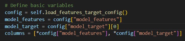
        config = self.load_features_target_config()
        model_features = config["model_features"]
        model_target = config["model_target"][0]
        columns = [*config["model_features"], *config["model_target"]]

        # Set up the dataframe used for training
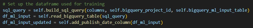
        sql_query = self.build_sql_query(columns, self.bigquery_project_id, self.bigquery_ml_input_table)
        df_ml_input = self.read_bigquery_table(sql_query)
        df_ml_input_updated = self.add_publish_date_column(df_ml_input)

        #  Split data into train and test sets based on dates
        df_train, df_test = self.split_data_by_date(df_ml_input_updated, cutoff_days)

        # Extract features and targets
        X_train, X_test, y_train, y_test = self.split_train_test(df_train, df_test, model_features, model_target)

        # Baseline model
        y_pred_baseline = self.baseline_model_predictions(df_train, y_test)
        mae_baseline, rmse_baseline = self.evaluate_model(y_test, y_pred_baseline)
        
        # XGBoost model
        xgb_model = self.build_xgboost_model(X_train, y_train)
        y_pred_xgb = xgb_model.predict(X_test)
        mae_xgb, rmse_xgb = self.evaluate_model(y_test, y_pred_xgb)
        self.save_model(xgb_model, "xgb_model")

        # LightGBM model
        lgb_model = self.build_lightgbm_model(X_train, y_train)
        y_pred_lgb = lgb_model.predict(X_test)
        mae_lgb, rmse_lgb = self.evaluate_model(y_test, y_pred_lgb)
        self.save_model(lgb_model, "lgb_model")

        return mae_baseline, rmse_baseline, mae_xgb, rmse_xgb, mae_lgb, rmse_lgb

The run() method puts everything together; since we’ve covered a lot, here’s a quick recap to solidify your understanding.

First, it loads and defines the model features and target from a yaml file:

Then it loads a dataset (created in Part II) from BigQuery and adds a publish_date column to make the train-test split possible:

As a next step, it divides the loaded dataset into train and test datasets:

Then it calculates and evaluates a baseline performance devoid of any ML solutions:

After that it builds an XGBoost and a LightGBM ML model and evaluates them:

Finally, it checks the results of each model (baseline vs ML models):

Now you can run the script. 🙂

WAIT!

Don’t do that. 😱

There’s a little caveat.

Read the next section to find out what I mean.

3. Making the models better by modifying the features

Do you remember this part earlier from the article?

What do you see?

Look close:

That’s a footnote.

Now.

You either 1) didn’t see it at the first time (that’s okay) or 2) you saw it but ignored it (still okay) or 3) saw it, clicked on it and read the footnote (cool!).

This is what the footnote says:

What? You noticed the features changed since the last article? Observant, aren’t you? Check out the “3. Making the models better by modifying the features” section – you’ll understand everything. 😉

Here’s the honest truth: I tweaked the features we created back in part II.

I’ve added a new one called title_is_highlights.

And I’ve deleted two (publish_is_weekend and publish_quarter).

Why would I do that?

See, building ML models is an iterative process.

You have some initial idea of what features to include in the train dataset, then you train your model and get some initial results which you’d like to improve further.

Using the feature importance plots shown above, I’ve seen that publish_is_weekend and publish_quarter both can be removed from the features since they bore no importance for the models.

I wasn’t happy with the initial performance of the models either.

So I did something that you should always try when engineering features: improve the input data.

(Because honestly, these models are already great, so a bit tweaking of the input data can yield huge performance increases.)

So I checked the videos again on YouTube:

I’ve seen some videos having an outstanding number of views (=millions) compared to others. Like this:

Or this:

And this:

What’s the common denominator?

They were all highlights!

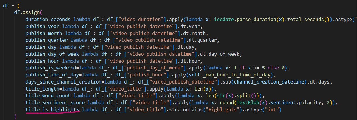
So I created a new feature called title_is_highlights whose value is 1 if the video title contains “Highlights” otherwise its value is 0.

This new feature made a huge difference in performance and became one of the top features in the dataset (see the feature importance plots above).

Moral of the story is that knowing your input data can help you build better ML models.

I added the new feature to ml-input-pipeline.py (script from part II):

I reran the script to get this new feature into my BigQuery table (ml-input):

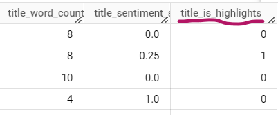
Notice how publish_is_weekend and publish_quarter are still in the table:

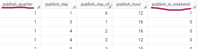
I just don’t use them in the script anymore because I’ve removed them from features_target_config.yaml:

See how useful yaml is? 🙂

Anyways, once you make these feature adjustments in your script, now you’re ready to run the ML model building script!

4. But how did the models perform?

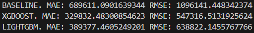
According to my results, both ML models beat the baseline prediction:

Without the title_is_highlights newly added feature, the results would’ve been this:

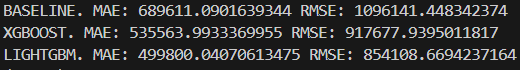
See how much the MAE and RMSE decreased for both XGBoost and LightGBM? 😎

Some background infos on my dataset and script settings:

my full dataset contains data for 3000 videos,
the train dataset contains 2268 examples (75.6%),
the test dataset contains 732 rows (24.4%),
both for the baseline calculation and the train-test split, I’ve used the default days values: 30 and 180 respectively.

Naturally, the created models are far from perfect and could be improved a lot by:

experimenting with hyperparameters,
engineering better features,
collecting more data for training,
or even trying other models.

Building useful ML models involve a lot more work, and I didn’t want to make this article any longer than necessary.

Also, the idea was to show the high-level parts of model building, how exciting it is to find performance gains and where model building fits into an ML project’s flow.

And we’re far from finished. 🙂

5. So what…?

You learned how to train, evaluate and compare ML models against a baseline by:

managing features from a yaml file,
improving model performance through a deeper understanding of your input data,
building both XGBoost and LightGBM models, evaluating and saving them,
and comparing their performance against a baseline.

That’s quite a lot.

And you did it! 👏

Next time, we’ll take things up a notch and make our approach more production-ready.

Anyways.

If you have any questions/comments, drop ‘em here, DM me on Substack or hit me up on LinkedIn!

And have an awesome day! ✌️

PREVIOUS ARTICLES FROM THE SERIES

OTHER ARTICLES YOU MAY LIKE

But who am I to tell you what to do? You can just read this article if you feel like it.

I deliberately named my function “split_train_test” so it wouldn’t be confused with scikit-learn’s “train_test_split” method.

Underhyped

Discussion about this post